
11 Capital Budgeting Decision Making

Learning Objectives LO
LO1 Determine the payback period for an investment
LO2 Compute the simple rate of return for an investment
LO3 Apply the time value of money concept by computing the present value of a sum of money
LO4 Compute the internal rate of return for an investment
LO5 Evaluate the acceptability of an investment project using the net present value method
LO6 Analyze capital budgeting decision making methods
Capital budgeting decision making
Managers are responsible for many decisions, some with short-term and others with long-term financial consequences. Projects and investments with long-term financial consequences are referred to as capital projects. Therefore, capital budgeting refers to the process of planning projects or making decisions that have a long-term effect on the organization. Examples of capital projects include investments in long-term assets such as vehicles, machines, facilities, or equipment; launching new products or services; and expanding operations.
Capital budgeting decision making is a critical managerial skill. Most organizations have limited resources and more potential capital projects than they can fund. For this reason, managers must be able to evaluate the alternatives and select the project that offers the most benefit to the organization. The ability to choose appropriate capital investments is an essential component of an organization’s long-term financial health and stability.
This chapter discusses four methods for making capital budgeting decisions—the payback period method, the simple rate of return method, the internal rate of return method, and the net present value method.
Payback period LO1
Payback period
The payback period is the length of time that it takes for a project to recover the initial cost from the net cash inflows generated by the project. The payback period is expressed in years. The formula to compute the payback period considers the investment required and the annual net cash inflow from the investment.
Investment required
The required investment is the cost of the project less the trade-in or salvage value received for any assets exchanged in the transaction. For example, assume that Jill decides to purchase a new car for $12,000. She receives $3,000 for trading in her old car. The required investment in the new car is $12,000 – 3,000 = $9,000.
Annual net cash inflow
Annual net cash inflow is the net cash inflows and cash outflows yielded by the investment. Cash inflows have a positive effect on cash, and cash outflows have a negative effect on cash. Revenue and cost savings are cash inflows, whereas expenses and costs are cash outflows. When considering an investment that generates revenue and costs, the annual net cash inflow is cash revenue less cash expenses. For an investment that generates cost savings and costs, the annual net cash inflow is cost savings less cash expenses.
It is important to note that net cash inflow is not the same as net operating income, although they are similar. Net cash inflow only includes cash revenues, cost savings, and cash expenses. Net operating income includes some non-cash expenses like depreciation expense. While depreciation is an expense, it is not a cash payment. Instead, it is the expense used to allocate the cost of a long-term asset over a period of time. Since the payback method uses annual net cash inflow, depreciation is not considered for this calculation. If net operating income is given, depreciation expense must be added back to arrive at annual net cash inflow.
When annual net cash inflow is the same every year, the formula in Exhibit 11-1 is used to compute the payback period.
Exhibit 11-1 Payback period formula

The payback period method is often used as an investment screening tool rather than a final selection tool. The advantage of the payback period method is that it can be used to screen several competing projects quickly. For example, some organizations prefer to invest in projects in which the investment is recovered within a specified period, such as 3 to 5 years. This tool can be used to identify investments that meet specific payback criteria.
The example of Ancient Cities Tours is used to illustrate the capital budgeting decision making tools presented in this chapter. Ancient Cities Tours offers complete tour packages to historically significant Mayan, Aztec, and Inca sites in Latin America. The company is headquartered in Peru. The company owns the headquarters building and the equipment–tour bus, riverboat, and van–used for tours originating from the Peru location. Maya is the owner-operator of Ancient Cities Tours.
Maya is considering replacing the company’s tour bus with an updated model. She narrowed her search to two models designed to handle the Peruvian landscape, the Diamond LX and the VIP Express. The Diamond LX is a standard-size tour bus. It costs less to purchase and operate but accommodates fewer passengers (35 seats). The VIP Express is an oversized model. It costs more to purchase and operate but accommodates more passengers (57 seats).
Ancient Cities Tours schedules 12 tours per year from the Peru location. The company averages 35 paid guests per tour at an average revenue of $520 per guest for the bus portion of the tour. If Maya purchases the Diamond LX (35 seats), the tours would be limited to 35 paid guests per tour due to seat capacity. The VIP Express (57 seats) can accommodate additional guests. If Maya purchases the VIP Express, she estimates that she can book an average of 42 guest per tour. Additional data about both models is given in Exhibit 11-2.
Exhibit 11-2 Data for tour bus investment alternatives


Refer to the data in Exhibit 11-2 for Ancient Cities Tours. The payback period is calculated as the investment required divided by the annual net cash inflow from the project. The data in Exhibit 11-2 gives net operating income, which includes deprecation expense. Depreciation expense is a non-cash expense. When net operating income is provided, depreciation expense is added back to arrive at net cash inflow. Net cash inflows for the Diamond LX and VIP Express are $126,000 ($73,000 + 53,000) and $148,680 ($76,980 + 71,700), respectively.
The Diamond LX model’s payback period is $690,000 / 126,000 = 5.48 years.
The VIP Express model’s payback period is $810,000 / 148,680 = 5.45 years.
Maya will recover the costs of both investments in approximately 5.5 years. As a general rule, a shorter payback period is preferable.
While the payback period method is easy to use, its disadvantages are significant. First, this method does not consider the actual profitability of a project. And second, this method does not consider the time value of money. The time value of money concept states that money available today is inherently worth more than an identical amount of money available in the future. The time value of money is explored in more detail later in this chapter.
Check your understanding LO1
Simple rate of return LO2
The simple rate of return method is a straightforward method used to compute an approximate rate of return for an investment or project. The formula to calculate the simple rate of return includes the investment required for the project and the annual net operating income or cost savings resulting from the project.
Investment required
The required investment is the project’s cost less the trade-in or salvage value received for any assets exchanged in the transaction. The investment required is the same input used to compute the payback period. Recall the example in which Jill purchases a new car for $12,000. She receives $3,000 for trading in her old car. The required investment in the new car is $12,000 – 3,000 = $9,000.
Annual net operating income
Annual net operating income resents the investment’s revenues less its expenses. Since this method uses annual net operating income, depreciation expense is included in the calculation. If annual net cash flow is given, depreciation expense must be calculated and subtracted from net annual cash flow to arrive at net operating income.
The formula to compute the simple rate of return is presented in Exhibit 11-3.
Exhibit 11-3 Simple rate of return formula
![]()
The simple rate of return method is often used as an investment screening tool rather than a final selection tool. The advantage of this method is that it can be used to screen several competing projects quickly. For example, some organizations prefer to invest in projects with a minimum rate of return. This tool can identify the investments that meet a specific minimum rate of return.
Refer to the data in Exhibit 11-2 for Ancient Cities Tours. The simple rate of return is calculated as the project’s annual net operating income divided by the investment required. The investment required and annual net operating income are provided in Exhibit 11-2.
The Diamond LX model’s simple rate of return is $73,000 / $690,000 = 10.6%
The VIP Express model’s simple rate of return is $76,980 / $810,000 = 9.5%
A higher simple rate of return is preferable. The simple rate of return for the Diamond LX model is 1.1% higher than the VIP Express model. While this is good information, especially during the initial screening phase, the simple rate of return method has limitations. Like the payback period, this method does not consider the time value of money. Another limitation is that the simple rate of return method does not consider the project’s useful life. And finally, this method can only be applied to investments that yield consistent operating income over the project’s life.
Video Illustration 11-1: Payback period and simple rate of return illustrated LO1
Isabella owns a small machine shop that develops prototypes for metal products. She would like to purchase a new machine capable of creating custom steel tools. She is considered two different models.
The A model would cost $420,000, generate $260,000 in annual cash revenues, and $120,000 in annual cash operating costs. The A model has a 10-year useful life.
The B model would cost $360,000, generate $180,000 in annual cash revenues, and $60,000 in annual cash operating cost. The B model has an 8-year useful life.
Compute the payback period and simple rate of return for both machines.
Exhibit 11-4 Template to compute payback period, simple rate of return, and video explanation.

Check your understanding LO2
Time value of money LO3
The time value of money concept states that money available today is inherently worth more than an identical amount of money available in the future. For example, $1,000,000 paid today is intrinsically worth more than $1,000,000 payable at the end of the year. There are two financial reasons for this.
The first factor is the concept of inflation. Inflation is an economic concept that measures the general increase in prices and the resulting decline in the purchasing value of money over a period of time. Inflation typically occurs gradually over a long period of time, so it is often ignored in capital budgeting decisions.
The second reason, interest or return on investment, is relevant to capital budgeting decisions. Money today is worth more than money in the future because it can be used today to generate interest or a return. Money available today can be invested in an interest-bearing investment or an organizational project yielding a return on that investment. For example, assume that $1,000,000 is available today and can be invested in a savings account yielding 3% interest. In this case, $1,000,000 today becomes $1,000,000 x 1.03 = $1,030,000 one year from now. Or, a business could invest $1,000,000 in a new product that yields a 15% return. The $1,000,000 investment today would be worth $1,150,000 one year from now.
Since the formula to calculate interest is constant (principal x rate x time), mathematical tables, known as present value and future value tables, have been developed to determine the discount factors for many different interest or return rates and time periods. The discount factors provided in the tables cover two types of present value calculations, lump sum and annuity.
Present value of a lump sum
The present value of a lump sum, often referred to as the present value of 1, is the present value of a single cash flow at some future point. For example, a company will receive $10,000 when they sell a machine in 10 years. This is a single cash flow of $10,000 that happens one time 10 years from now.
Present value of an ordinary annuity
An annuity is a series of equal payments over multiple periods. An ordinary annuity is a series of payments in which the cash flows begin at the end of the time period. An annuity due is a series of payments in which the cash flows begin at the beginning of the time period. For example, assume a judicial settlement ordered annual payments of $100,000 per year for 5 years. The first payment will be disbursed one year from the settlement date. This settlement is an ordinary annuity. The undiscounted cash value of the settlement is $500,000 (5 payments x $100,000). However, because of the time value of money concept, the settlement is not valued at $500,000 since it is not fully payable now. The cash received in the second year is worth less than the cash received in the first year. And the cash received in the fifth year is worth less than the cash received in the first four years.
The present value of a lump sum and the present value of an ordinary annuity discount tables are provided in Appendix A: Present Value Tables. The discount factor provided in the tables can be used to easily determine the present value of a future lump sum or ordinary annuity amount. To find the present value, the future amount is multiplied by the discount factor for the corresponding interest rate and time period.
Check your understanding LO3
Internal rate of return LO4
The internal rate of return (IRR) method is similar to the simple rate of return with one significant difference. The IRR method takes into consideration the time value of money. This method calculates the discounted rate of return of an investment over the useful life of the investment. The formula to calculate IRR includes the investment required for the project and the annual net cash inflow from the project.
Investment required
The required investment is the project’s cost less the trade-in or salvage value received for any assets exchanged in the transaction. The investment required is the same input used for the payback period and the simple rate of return. Recall the example in which Jill purchases a new car for $12,000. She receives $3,000 for trading in her old car. The required investment in the new car is $12,000 – 3,000 = $9,000.
Annual net cash inflow
Annual net cash inflow is the net cash inflow yielded by the investment. Annual net cash inflow is also used for the payback period method. It is important to note that both revenue and cost savings are considered cash inflows. When considering an investment generating revenues and costs, annual net cash inflow is the cash revenue less cash costs. Since this method uses annual net cash inflow, depreciation expense is not considered for this calculation. If net income is given, depreciation expense must be added back to arrive at annual net cash inflow. When considering an investment generating cost savings and costs, annual net cash inflow is the cost savings less cash costs.
The formula to compute the discount factor used for the internal rate of return method is presented in Exhibit 11-5.
Exhibit 11-5 Present value of annuity discount factor formula
![]()
The formula in Exhibit 11-5 produces the investment’s discount factor. The discount factor is used to find the investment’s internal rate of return. To find the rate of return, locate the row matching the useful life of the project on the present value of an annuity discount table (Appendix A: Present Value Tables). Scan the useful life row to locate the number that is closest to the discount factor provided by the formula. The corresponding interest rate is the investment’s IRR.
The advantage of the internal rate of return over the payback method or the simple rate of return method is that IRR considers the time value of money. The major disadvantage is that IRR only works for investments with a single cash investment at the beginning and constant cash flows over the life of the investment. Many capital budgeting projects require multiple investments at different times during the project and produce uneven cash flows over the life of the investment.
Refer to the data in Exhibit 11-2 for Ancient Cities Tours. Computing the IRR is a two-step process. The first step is to use the formula to find the present value of an annuity discount factor. This formula is the same as the payback period formula. The present value of an annuity discount factor is calculated as the investment required divided by the annual net cash inflow from the project. The data in Exhibit 11-2 gives net operating income, which includes depreciation expense. Depreciation expense is a non-cash expense. When net operating income is given, depreciation expense is added back to arrive at net cash inflow. Net cash inflows for the Diamond LX and VIP Express are $126,000 ($73,000 + 53,000) and $148,680 ($76,980 + 71,700), respectively.
Diamond LX model’s present value of an annuity discount factor is $690,000 / 126,000 = 5.48.
VIP Express model’s present value of an annuity discount factor is $810,000 / 148,680 = 5.45.
The second step is to locate the discount factor on the present value of an annuity discount table (Appendix A: Present Value Tables) in the row matching the project’s useful life. The corresponding rate of return is the internal rate of return. The useful lives are given in Exhibit 11-2 as 12 years for the Diamond LX and 10 years for the VIP Express.
For the Diamond LX model, the discount factor closest to 5.48 on row 12 (years useful life) is 5.421. This corresponds with a 15% internal rate of return.
For the VIP Express model, the discount factor closest to 5.45 on row 10 (years useful life) is 5.426. This corresponds with a 13% internal rate of return.
A higher internal rate of return is preferable. The IRR for the Diamond LX model is 2% higher than the VIP Express model. As demonstrated in the preceding section, the simple rate of return for the Diamond LX model is 1.1% higher than the VIP Express model. The IRR is more accurate than the simple rate of return because it considers the time value of money as well as the useful life of the projects.
However, the internal rate of return method has limitations. A significant limitation is that this method assumes that the revenue and expenses generated by the investment are constant over the project’s life. Additionally, this method only considers the initial investment and the annual net cash inflows. This method does not consider other cash inflows or cash outflows, such as any salvage value for the project at the end of its useful life.
Video Illustration 11-2: Internal rate of return LO4
Paula is thinking about replacing her stitching machine. A new machine would cost $130,000. She would receive $6,000 for trading in her old machine. The new machine would generate $52,000 in annual revenue and $27,000 in annual cash expenses. The new machine has an 8 year useful life.
What is the internal rate of return for the new stitching machine?
Check your understanding LO4
Net present value method (NPV) LO5
The net present value method compares the present value of a project’s cash inflows to the present value of its cash outflows at a predetermined discount rate. The discount rate is the minimum rate of return established by the organization. All the cash inflows and outflows from an investment are discounted at this rate. Discounted cash inflows are positive, and discounted cash outflows are negative. The discounted cash flows are then netted together to produce the investment’s net present value.
Like the internal rate of return method, the net present value method considers the time value of money. Unlike the internal rate of return method, the net present value method can be used to evaluate investments where multiple cash investments are required, or the project has uneven cash flows over the life of the investment.
Positive net present value
A positive net present value means that the return on the investment is greater than the discount rate. Or that the investment yields a higher return than the discount rate used in the analysis. For example, if the net present value is positive and the discount rate is 12%, the project returns more than 12%. Although this tool does not provide the exact return, a positive value means that the return is more than 12%.
Zero net present value
A zero net present value means that the return on the investment equals the discount rate. A zero net present value does not mean the investment has a zero return. The cash flows were discounted at a specific rate so the investment returns exactly that rate. For example, if the net present value is zero and the discount rate used is 12%, the project returns exactly 12%.
Negative net present value
A negative net present value means that the return on the investment is less than the discount rate. Or that the investment yields a lower return than the discount rate. This does not mean that the investment does not generate a return. Instead, it means that the return is less than the discount rate. For example, if the net present value is negative and the discount rate is 12%, the project returns less than 12%. Although this tool does not provide the exact return, a negative value means that the return is less than 12%.
Refer to the data in Exhibit 11-2 for Ancient Cities Tours. Assume that the discount rate for Ancient Cities Tours is 10%. The net present value method calculates the present value for all cash flows associated with the two models. The net present values for the tour bus alternatives are provided in Exhibit 11-6.
Exhibit 11-6 Net present values for the tour bus alternatives
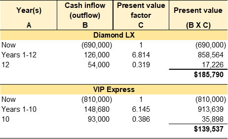
Refer to the data in Exhibit 11-6.
Column B lists the cash inflows and outflows for the project or investment. Cash inflows are positive, and cash outflows are negative.
Column A is for the year or years in which the cash inflow or outflow occurs. There are three options for this column. Now is used for cash inflows or outflows that happen immediately. An annuity is a series of equal payments entered as years x to x. A lump sum is a single receipt or cash payment in the future entered as a single year.
Column C is for the present value factor from the present value tables (Appendix A: Present Value Tables). Use the present value of an annuity chart for a series of payments, e.g., years x to x. Use the present value of a lump sum chart for a single lump sum payment.
Column D is the present value of the cash inflow or outflow (column B x column C).
The Diamond LX and VIP Express models have the same types of cash inflows/outflows–investment required, annual net cash inflows, and the salvage value at the end of the useful life. The discount rate for Ancient Cities Tours is 10%.
The original investment represents an immediate cash outflow. The year is now since it will be spent immediately. The discount factor for an immediate cash inflow or outflow is 1 since the time value of an amount today is 100%. Or, $1 today is worth $1.
The annual net cash inflows are positive since this is the net cash received from the investment. The useful life for the Diamond LX and VIP Express models are 12 and 10 years, respectively. The annual net cash inflows are a series of cash receipts. Accordingly, the discount factor is selected from the present value of an ordinary annuity table. The Diamond LX discount factor is 6.814 taken from row 12, 10% column. The VIP Express discount factor is 6.145 taken from row 10, 10% column.
Salvage value is the residual value of an investment or asset at the end of its useful life. It represents the amount the organization can realize if they sell or trade the asset at the end of its useful life. For example, Maya estimates that she can sell the Diamond LX for $54,000 in 12 years and the VIP Express for $93,000 in 10 years. Salvage value is a cash inflow, so it is positive. Since this is a lump sum cash inflow at the end of the asset’s useful life, the discount factor is selected from the present value of a lump sum table. The Diamond LX discount factor is 0.319 taken from row 12, 10% column. The VIP Express discount factor is 0.386 taken from row 10, 10% column.
The present value of each cash inflow and outflow is calculated in column D (column B x column C). The investment’s net present value is the sum of the present value for the cash inflows and outflows. Both models have a positive net present value, meaning they return over 10%. A zero net present value would mean the model returned precisely 10%. And a negative net present value means the models did not return 10%. It is important to note that a negative net present value does not always mean the project has a negative return. Instead, it indicates that the project does not return the discount rate used for the analysis. In this example, the net cash inflows from the Diamond LX model have a slightly higher net present value than the net cash inflows from the VIP Express model.
Video Illustration 11-3: Net present value method LO5
Jen Labs is considering the purchase of a new lab machine to test blood samples for specific viruses. The machine costs $372,000. The machine has a useful life of 6 years. The machine will require a $50,000 general maintenance service in year 3. If they purchase this machine, they estimate that they will run 1,500 blood tests per year. They can charge $120 per blood test. The machine will require $81,000 per year in operating costs. At the end of the six years, the machine has a $24,000 trade-in value. Jen Labs requires a minimum return of 10% on all investments.
Compute the net present value of this investment using Appendix A: Present Value Tables.
Exhibit 11-7 Template to compute net present value and video explanation.
Check your understanding L05
Analyzing capital budgeting decision making methods LO6
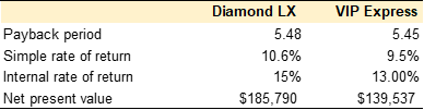
The capital budgeting decision making methods introduced in this chapter are used to analyze capital purchases or investments. A summary of the analysis for Ancient Cities Tours is presented in Exhibit 11-8. The Diamond LX model has a higher simple rate of return, internal rate of return, and net present value. The payment periods for both models are essentially the same. Based solely on this analysis, the Diamond LX is the better alternative.
Exhibit 11-8 Summary Ancient Cities Tours capital budgeting decision making methods using original data
It is important to emphasize that the analysis in Exhibit 11-8 is based on the estimates and projections given in the original data in Exhibit 11-2. Assume that the manufacturer provided each model’s estimated useful life. Maya determined that both models could be used for 12 years. Changing this assumption will affect the simple rate of return, internal rate of return, and net present value results. A summary of the results using a 12-year useful life for both models is presented in Exhibit 11-9. The VIP Express is the better alternative when a 12-year useful life is used for both models.
Exhibit 11-9 Summary Ancient Cities Tours capital budgeting decision making methods assuming 12-year useful life.

As demonstrated, the capital budgeting decision making methods presented in this chapter are practical tools for evaluating capital projects or investments. The results, however, depend on the accuracy and quality of the estimates and projection data inputted into the methods.
Practice Video Problems
The chapter concepts are applied to comprehensive business scenarios in the below Practice Video Problems.
Practice Video Problem 11-1: Payback period, simple rate of return, and internal rate of return LO1, LO2, LO3
Holly Rich is considering becoming an independent contractor for a national rideshare company as a second job. Her current car is older and not reliable enough to use for the business. She is considering purchasing a newer car to use in the business. A reliable used car would cost $19,000. The dealer offered her $1,000 trade-in value on her old car. The trade-in will be applied to the purchase of the new car. The car will have a 5-year useful life. She estimates that she can provide 40 rides per week and work 50 weeks per year. She earns an average of $9 per ride. Her cash expenses average $6.50 per ride. Annual depreciation on the car would be $3,800 per year.
Required: Compute the payback period, simple rate of return, and internal rate of return for this investment.
Payback period
Simple rate of return
Internal rate of return
Practice Video Problem 11-2: Net present value method LO6
The manager of Quick Print, Inc. wants to replace an outdated, large-format analog printer. She has narrowed the decision down to two digital models, the standard commercial model or the premium commercial model. The required minimum rate of return on all investments is 12%.
The standard model costs $72,000 and has a useful life of 6 years. The standard model requires maintenance service in year 2 and year 4 at a cost of $2,100 per service. Annual revenue is estimated to be $36,000 and annual cash operating expenses are estimated to be $12,000. The salvage value is estimated to be $7,200.
The premium model cost $93,000 and has a useful life of 8 years. The premium model requires maintenance service in year 2, year 4, and year 6 at a cost of $2,100 per service. This copier can be used to provide more services than the standard model so annual revenue is estimated to be $52,000 and annual cash operating expenses are estimated to be $21,000. The salvage value is estimated to be $5,200.
Required: Compute the net present value for both copiers using Appendix A: Present Value Tables.
Review Questions
Review questions reinforce the chapter content.
LO5: Evaluate the acceptability of an investment project using the net present value method
Homework Questions
Homework questions can be used for additional practice or can be assigned in an academic setting. Full feedback is not available online. Homework questions can be assigned, with auto-grading and export, to specific learning management platforms, e.g., Canvas, Blackboard, etc. Contact the author for details.
LO5: Evaluate the acceptability of an investment project using the net present value method
